Using supplychainpy with Pandas, Jupyter and Matplotlib
The following is taken from the jupyter notebook title ‘0.0.4-Using-Supplychainpy-and-Pandas-v1’ found here . For a more interactive experience please retrieve this notebook and run with jupyter.
To use supplychainpy with Pandas, we first read a csv file to a Pandas DataFrame.
%matplotlib inline

import matplotlib
import pandas as pd

from supplychainpy.model_inventory import analyse
from supplychainpy.model_demand import simple_exponential_smoothing_forecast
from supplychainpy.sample_data.config import ABS_FILE_PATH

raw_df =pd.read_csv(ABS_FILE_PATH['COMPLETE_CSV_SM'])
print(raw_df)
          Sku   jan   feb   mar   apr   may   jun   jul   aug   sep   oct  0   KR202-209  1509  1855  2665  1841  1231  2598  1988  1988  2927  2707
1   KR202-210  1006   206  2588   670  2768  2809  1475  1537   919  2525
2   KR202-211  1840  2284   850   983  2737  1264  2002  1980   235  1489
3   KR202-212   104  2262   350   528  2570  1216  1101  2755  2856  2381
4   KR202-213   489   954  1112   199   919   330   561  2372   921  1587
5   KR202-214  2416  2010  2527  1409  1059   890  2837   276   987  2228
6   KR202-215   403  1737   753  1982  2775   380  1561  1230  1262  2249
7   KR202-216  2908   929   684  2618  1477  1508   765    43  2550  2157
8   KR202-217  2799  2197  1647  2263   224  2987  2366   588  1140   869
9   KR202-218  1333   402   804   318  1408   830  1028   534  1871  2730
10  KR202-219   813   969   745  1001  2732  1987   717   599  2722   171
11  KR202-220  1481   905  1067  2513   861  1670   650  2630  1245   997
12  KR202-221   771  2941  1360  2714  1801  1744  1428  1660   436   578
13  KR202-222  2349     4   345   524   340  2698  2137  1164   498  1583
14  KR202-223  2045  2055   552    81  2780   176  2316  1475  2566  1678
15  KR202-224  2482  1887  1911  1446  2939  1241  1281   692   119   627
16  KR202-225  2744  2770  2697  1726  1776  2264   332  2420  2722  1161
17  KR202-226  2509   914   903   877  1859  2263   383   593   236   189
18  KR202-227   368  2502  2955  2994  1270  2884  2208   699   854   877
19  KR202-228  1468  1109  2464  2799   948   589  2858  1140   501  2691
20  KR202-229  2114   198  1479  1249  1475   744   407  2280   226  2285
21  KR202-230  1023  1150  1672  2026  1590   441  2484  2300  2928  1082
22  KR202-231   482   546   299  2304  2953  1029  1863  2809   454   927
23  KR202-232   614  2138   962  2017  2398  2963  2189  1804   414  2016
24  KR202-233  2395  2521  2157   728  1028    43   138   826   570  2825
25  KR202-234  1336  1478   865   533  1562   422  2287  1302  1230  1059
26  KR202-235  2565  2762  2721  1431   845  2163  2413  2227  1753   740
27  KR202-236  1912  1726  1569   316    71  2082   108   174  1974   609
28  KR202-237  2153  1112    16   130   590  2619  2576  2390  2567  1531
29  KR202-238  1417  2044  1981  1936  2377   780  1544  1521    51  1056
30  KR202-239  2717  2186  2300   677  2157  2328  1917  2519   561   281
31  KR202-240  1015   741  2754  2925  2302   695  2869   440   406  1083
32  KR202-241  3050  1507  3637  1112  1963  1675   898  1986  2262  3895
33  KR202-242  1875  2368   830   823   868  1409  1845  3095  3247  1894
34  KR202-243  1717   593  3006  2935  3139  2753  3247  3845  1720  3413
35  KR202-244  2383  2046  2487  3827  1674  3118  2849  2233  3888  2566
36  KR202-245  1115  2694  3038  3366  1058  2724  2863  1930  1787   838
37  KR202-246  3108  1197  2472  1264  3179  3638  1268  1581  3456  1630
38  KR202-247  3439  1854   652  1827  1645  2257  2733  1337  2034  2106

     nov   dec  unit cost  lead-time  retail_price  quantity_on_hand  backlog
0    731  2598       1001          2          5000              1003       10
1    440  2691        394          2          1300              3224       10
2    218   525        434          4          1200               390       10
3   1867  2743        474          3            10               390       10
4   1532  1512        514          1          2000              2095       10
5   1095  1396        554          2          1800                55       10
6    824   743        594          1          2500              4308       10
7    937  1201        634          3          3033                34       10
8   1707  1180        674          3          5433               390       10
9   2022    94        714          2          3034              3535       10
10   639  2108        754          3          5000               334       10
11  1936  2780        794          3          7500              3434       10
12  1956  1101        834          2          4938              4433       10
13  1241  2965        874          2          4922              3435       10
14  1553  2745        914          1          4894             34533       10
15  1941  1383        954          2          2942                33       10
16  1986  2587        994          6          8999              2000       10
17   920  1686       1034          3          4342              4344       10
18  2320   160       1074          3          4920               489       10
19    93  1060       1114          2         15000              9439       10
20   796  1948       1154          2         13000              8939       10
21  2064  2412       1194          2         10000               349       10
22  2488  2341       1234          4          9999              3434       10
23  1350  2464       1274          2          7500               234       10
24   181   787       1314          4          6000               349       10
25  1153   399       1354          2         20000               324       10
26  1139  2300       1394          3         59500               850       10
27  2896   566       1434          3          2300              4930       10
28   842   242       1474          2          4500              9483       10
29  1876  1356       1514          3          8000               839       10
30  1162  1146       1554          2         39000               433       10
31  2334  1015       1594          3          3943               390       10
32  1229  2904        769          5          8007              2125       10
33  2558  3048       1819          1         13225              1253       10
34  3399  2799       1120          3         14682              1128       10
35  2216  3817       1067          5         11997              1191       10
36  3087  1565       1623          2         12876               611       10
37  1788  2288        608          2          6548              2192       10
38   877  2409       1578          2         10463              1017       10
Passing a Pandas DataFrame as a keyword parameter (df=) returns a
DataFrame with the inventory profile analysed. Excluding the import
statements this can be achieved in 3 lines of code. There are several
columns, so the print statement has been limited to a few.
orders_df = raw_df[['Sku','jan','feb','mar','apr', 'may', 'jun', 'jul', 'aug', 'sep', 'oct', 'nov', 'dec']]
#orders_df.set_index('Sku')
analysis_df = analyse(df=raw_df, start=1, interval_length=12, interval_type='months')
print(analysis_df[['sku','quantity_on_hand', 'excess_stock', 'shortages', 'ABC_XYZ_Classification']])
          sku quantity_on_hand excess_stock shortages ABC_XYZ_Classification
0   KR202-209             1003            0      5969                     BY
1   KR202-210             3224            0         0                     CY
2   KR202-211              390            0      7099                     CY
3   KR202-212              390            0      7759                     CY
4   KR202-213             2095            0         0                     CY
5   KR202-214               55            0      5824                     CY
6   KR202-215             4308          732         0                     CY
7   KR202-216               34            0      6999                     CY
8   KR202-217              390            0      7245                     BY
9   KR202-218             3535            0         0                     CZ
10  KR202-219              334            0      5917                     CZ
11  KR202-220             3434            0         0                     BY
12  KR202-221             4433            0         0                     BY
13  KR202-222             3435            0         0                     CZ
14  KR202-223            34533        30030         0                     BY
15  KR202-224               33            0      5580                     CY
16  KR202-225             2000            0     10542                     AY
17  KR202-226             4344            0         0                     CZ
18  KR202-227              489            0      7587                     BZ
19  KR202-228             9439         3572         0                     AZ
20  KR202-229             8939         3994         0                     AY
21  KR202-230              349            0      5913                     AY
22  KR202-231             3434            0         0                     AZ
23  KR202-232              234            0      6150                     AY
24  KR202-233              349            0      6856                     CZ
25  KR202-234              324            0      3822                     AY
26  KR202-235              850            0      7339                     AY
27  KR202-236             4930            0         0                     CZ
28  KR202-237             9483         3742         0                     CZ
29  KR202-238              839            0      5693                     BY
30  KR202-239              433            0      5737                     AY
31  KR202-240              390            0      7094                     CZ
32  KR202-241             2125            0     10328                     AY
33  KR202-242             1253            0         0                     AY
34  KR202-243             1128            0     10227                     AY
35  KR202-244             1191            0     13200                     AY
36  KR202-245              611            0      7081                     AY
37  KR202-246             2192            0         0                     AY
38  KR202-247             1017            0      5776                     AY
Before we can make a forecast we need to select a SKU from the
analysis_df variable, slice the row to retrive only orders data and
convert to a Series.
row_ds = raw_df[raw_df['Sku']=='KR202-212'].squeeze()
print(row_ds[1:12])
jan     104
feb    2262
mar     350
apr     528
may    2570
jun    1216
jul    1101
aug    2755
sep    2856
oct    2381
nov    1867
Name: 3, dtype: object
Now that we have a series of orders data fro the SKU KR202-212,
we can now perform a forecast using the model_demand module. We can
perform a simple_exponential_smoothing_forecast by passing the
forecasting function the orders data using the keyword parameter
ds=.
ses_df = simple_exponential_smoothing_forecast(ds=row_ds[1:12], length=12, smoothing_level_constant=0.5)
print(ses_df)
{'statistics': {'pvalue': 0.0047852515832242743, 'test_statistic': 3.8634855288615153, 'std_residuals': 4793.7283216530095, 'intercept': 377.59999999999991, 'trend': True, 'slope': 224.4909090909091, 'slope_standard_error': 58.105797838218294}, 'alpha': 0.5, 'forecast_breakdown': [{'squared_error': 2345353.024793389, 'alpha': 0.5, 'demand': 104, 'one_step_forecast': 1635.4545454545455, 't': 1, 'level_estimates': 869.72727272727275, 'forecast_error': -1531.4545454545455}, {'squared_error': 1938423.3471074379, 'alpha': 0.5, 'demand': 2262, 'one_step_forecast': 869.72727272727275, 't': 2, 'level_estimates': 1565.8636363636365, 'forecast_error': 1392.2727272727273}, {'squared_error': 1478324.3822314052, 'alpha': 0.5, 'demand': 350, 'one_step_forecast': 1565.8636363636365, 't': 3, 'level_estimates': 957.93181818181824, 'forecast_error': -1215.8636363636365}, {'squared_error': 184841.36828512402, 'alpha': 0.5, 'demand': 528, 'one_step_forecast': 957.93181818181824, 't': 4, 'level_estimates': 742.96590909090912, 'forecast_error': -429.93181818181824}, {'squared_error': 3338053.5693440083, 'alpha': 0.5, 'demand': 2570, 'one_step_forecast': 742.96590909090912, 't': 5, 'level_estimates': 1656.4829545454545, 'forecast_error': 1827.034090909091}, {'squared_error': 194025.23324509294, 'alpha': 0.5, 'demand': 1216, 'one_step_forecast': 1656.4829545454545, 't': 6, 'level_estimates': 1436.2414772727273, 'forecast_error': -440.4829545454545}, {'squared_error': 112386.84808400051, 'alpha': 0.5, 'demand': 1101, 'one_step_forecast': 1436.2414772727273, 't': 7, 'level_estimates': 1268.6207386363635, 'forecast_error': -335.24147727272725}, {'squared_error': 2209323.3086119094, 'alpha': 0.5, 'demand': 2755, 'one_step_forecast': 1268.6207386363635, 't': 8, 'level_estimates': 2011.8103693181818, 'forecast_error': 1486.3792613636365}, {'squared_error': 712656.13255070464, 'alpha': 0.5, 'demand': 2856, 'one_step_forecast': 2011.8103693181818, 't': 9, 'level_estimates': 2433.905184659091, 'forecast_error': 844.18963068181824}, {'squared_error': 2798.9585638125168, 'alpha': 0.5, 'demand': 2381, 'one_step_forecast': 2433.905184659091, 't': 10, 'level_estimates': 2407.4525923295455, 'forecast_error': -52.905184659090992}, {'squared_error': 292089.0045557259, 'alpha': 0.5, 'demand': 1867, 'one_step_forecast': 2407.4525923295455, 't': 11, 'level_estimates': 2137.226296164773, 'forecast_error': -540.4525923295455}], 'mape': 100.69830747447692, 'forecast': [2137.226296164773, 2137.226296164773, 2137.226296164773, 2137.226296164773, 2137.226296164773]}
print(ses_df.get('forecast', 'UNKNOWN'))
[2137.226296164773, 2137.226296164773, 2137.226296164773, 2137.226296164773, 2137.226296164773]
If we check the statistcs for the forecast we can see whether there is a linear trend and subsequently if the forecast is useful.
print(ses_df.get('statistics', 'UNKNOWN'),'\n mape: {}'.format(ses_df.get('mape', 'UNKNOWN')))
{'pvalue': 0.0047852515832242743, 'test_statistic': 3.8634855288615153, 'std_residuals': 4793.7283216530095, 'intercept': 377.59999999999991, 'trend': True, 'slope': 224.4909090909091, 'slope_standard_error': 58.105797838218294}
 mape: 100.69830747447692
The breakdown of the forecast is also returned with the forecast and
statistics.
print(ses_df.get('forecast_breakdown', 'UNKNOWN'))
[{'squared_error': 2345353.024793389, 'alpha': 0.5, 'demand': 104, 'one_step_forecast': 1635.4545454545455, 't': 1, 'level_estimates': 869.72727272727275, 'forecast_error': -1531.4545454545455}, {'squared_error': 1938423.3471074379, 'alpha': 0.5, 'demand': 2262, 'one_step_forecast': 869.72727272727275, 't': 2, 'level_estimates': 1565.8636363636365, 'forecast_error': 1392.2727272727273}, {'squared_error': 1478324.3822314052, 'alpha': 0.5, 'demand': 350, 'one_step_forecast': 1565.8636363636365, 't': 3, 'level_estimates': 957.93181818181824, 'forecast_error': -1215.8636363636365}, {'squared_error': 184841.36828512402, 'alpha': 0.5, 'demand': 528, 'one_step_forecast': 957.93181818181824, 't': 4, 'level_estimates': 742.96590909090912, 'forecast_error': -429.93181818181824}, {'squared_error': 3338053.5693440083, 'alpha': 0.5, 'demand': 2570, 'one_step_forecast': 742.96590909090912, 't': 5, 'level_estimates': 1656.4829545454545, 'forecast_error': 1827.034090909091}, {'squared_error': 194025.23324509294, 'alpha': 0.5, 'demand': 1216, 'one_step_forecast': 1656.4829545454545, 't': 6, 'level_estimates': 1436.2414772727273, 'forecast_error': -440.4829545454545}, {'squared_error': 112386.84808400051, 'alpha': 0.5, 'demand': 1101, 'one_step_forecast': 1436.2414772727273, 't': 7, 'level_estimates': 1268.6207386363635, 'forecast_error': -335.24147727272725}, {'squared_error': 2209323.3086119094, 'alpha': 0.5, 'demand': 2755, 'one_step_forecast': 1268.6207386363635, 't': 8, 'level_estimates': 2011.8103693181818, 'forecast_error': 1486.3792613636365}, {'squared_error': 712656.13255070464, 'alpha': 0.5, 'demand': 2856, 'one_step_forecast': 2011.8103693181818, 't': 9, 'level_estimates': 2433.905184659091, 'forecast_error': 844.18963068181824}, {'squared_error': 2798.9585638125168, 'alpha': 0.5, 'demand': 2381, 'one_step_forecast': 2433.905184659091, 't': 10, 'level_estimates': 2407.4525923295455, 'forecast_error': -52.905184659090992}, {'squared_error': 292089.0045557259, 'alpha': 0.5, 'demand': 1867, 'one_step_forecast': 2407.4525923295455, 't': 11, 'level_estimates': 2137.226296164773, 'forecast_error': -540.4525923295455}]
We can convert the forecast_breakdown back into a DataFrame.
forecast_breakdown_df = pd.DataFrame(ses_df.get('forecast_breakdown', 'UNKNOWN'))
print(forecast_breakdown_df)
    alpha  demand  forecast_error  level_estimates  one_step_forecast  0     0.5     104    -1531.454545       869.727273        1635.454545
1     0.5    2262     1392.272727      1565.863636         869.727273
2     0.5     350    -1215.863636       957.931818        1565.863636
3     0.5     528     -429.931818       742.965909         957.931818
4     0.5    2570     1827.034091      1656.482955         742.965909
5     0.5    1216     -440.482955      1436.241477        1656.482955
6     0.5    1101     -335.241477      1268.620739        1436.241477
7     0.5    2755     1486.379261      2011.810369        1268.620739
8     0.5    2856      844.189631      2433.905185        2011.810369
9     0.5    2381      -52.905185      2407.452592        2433.905185
10    0.5    1867     -540.452592      2137.226296        2407.452592

    squared_error   t
0    2.345353e+06   1
1    1.938423e+06   2
2    1.478324e+06   3
3    1.848414e+05   4
4    3.338054e+06   5
5    1.940252e+05   6
6    1.123868e+05   7
7    2.209323e+06   8
8    7.126561e+05   9
9    2.798959e+03  10
10   2.920890e+05  11
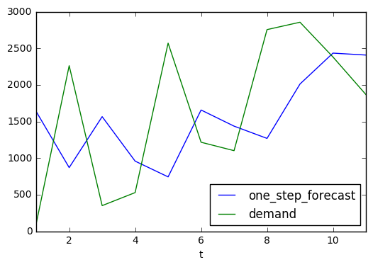
Let’s look at the demand and the one_step_forecast in a chart.
forecast_breakdown_df.plot(x='t', y=['one_step_forecast','demand'])
<matplotlib.axes._subplots.AxesSubplot at 0x10e1be400>
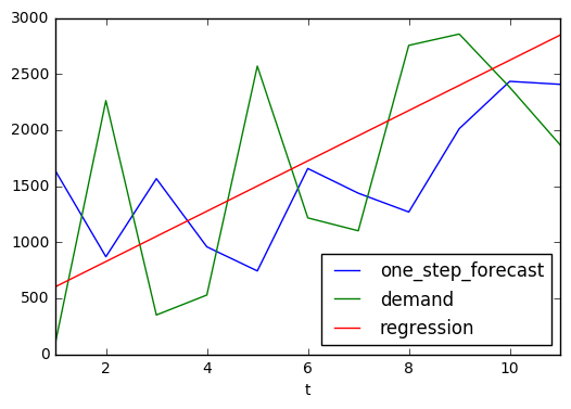
Using y = mx + c we can also create the data points for the
regression line.
regression = {'regression': [(ses_df.get('statistics')['slope']* i ) + ses_df.get('statistics')['intercept'] for i in range(1,12)]}
print(regression)
{'regression': [602.09090909090901, 826.58181818181811, 1051.0727272727272, 1275.5636363636363, 1500.0545454545454, 1724.5454545454545, 1949.0363636363636, 2173.5272727272727, 2398.0181818181818, 2622.5090909090909, 2847.0]}
We can add the regression data points to the forecast breakdwn DataFrame.
forecast_breakdown_df['regression'] = regression.get('regression')
print(forecast_breakdown_df)
    alpha  demand  forecast_error  level_estimates  one_step_forecast  0     0.5     104    -1531.454545       869.727273        1635.454545
1     0.5    2262     1392.272727      1565.863636         869.727273
2     0.5     350    -1215.863636       957.931818        1565.863636
3     0.5     528     -429.931818       742.965909         957.931818
4     0.5    2570     1827.034091      1656.482955         742.965909
5     0.5    1216     -440.482955      1436.241477        1656.482955
6     0.5    1101     -335.241477      1268.620739        1436.241477
7     0.5    2755     1486.379261      2011.810369        1268.620739
8     0.5    2856      844.189631      2433.905185        2011.810369
9     0.5    2381      -52.905185      2407.452592        2433.905185
10    0.5    1867     -540.452592      2137.226296        2407.452592

    squared_error   t   regression
0    2.345353e+06   1   602.090909
1    1.938423e+06   2   826.581818
2    1.478324e+06   3  1051.072727
3    1.848414e+05   4  1275.563636
4    3.338054e+06   5  1500.054545
5    1.940252e+05   6  1724.545455
6    1.123868e+05   7  1949.036364
7    2.209323e+06   8  2173.527273
8    7.126561e+05   9  2398.018182
9    2.798959e+03  10  2622.509091
10   2.920890e+05  11  2847.000000
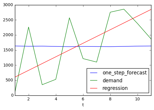
forecast_breakdown_df.plot(x='t', y=['one_step_forecast','demand', 'regression'])
<matplotlib.axes._subplots.AxesSubplot at 0x110a83b38>
We have a choice now, we can use another alpha and repeat the analysis
to reduce the Standard Error or use supplychainpy’s optimise=True
parameter to use an evolutionary algorithm and get closer to an optimal
solution.
opt_ses_df = simple_exponential_smoothing_forecast(ds=row_ds[1:12], length=12, smoothing_level_constant=0.4,optimise=True)
print(opt_ses_df)
{'statistics': {'pvalue': 0.0047852515832242743, 'test_statistic': 3.8634855288615153, 'std_residuals': 4793.7283216530095, 'intercept': 377.59999999999991, 'trend': True, 'slope': 224.4909090909091, 'slope_standard_error': 58.105797838218294}, 'optimal_alpha': 0.006889829296806371, 'mape': 209.37388042679993, 'standard_error': 1097.3575476759161, 'forecast_breakdown': [{'squared_error': 2345353.024793389, 'alpha': 0.006889829296806371, 'demand': 104, 'one_step_forecast': 1635.4545454545455, 't': 1, 'level_estimates': 1624.9030850605454, 'forecast_error': -1531.4545454545455}, {'squared_error': 405892.47902537062, 'alpha': 0.006889829296806371, 'demand': 2262, 'one_step_forecast': 1624.9030850605454, 't': 2, 'level_estimates': 1629.2925740500002, 'forecast_error': 637.09691493945456}, {'squared_error': 1636589.4900194753, 'alpha': 0.006889829296806371, 'demand': 350, 'one_step_forecast': 1629.2925740500002, 't': 3, 'level_estimates': 1620.4784665941236, 'forecast_error': -1279.2925740500002}, {'squared_error': 1193509.1999718475, 'alpha': 0.006889829296806371, 'demand': 528, 'one_step_forecast': 1620.4784665941236, 't': 4, 'level_estimates': 1612.9514764488533, 'forecast_error': -1092.4784665941236}, {'squared_error': 915941.87643142976, 'alpha': 0.006889829296806371, 'demand': 2570, 'one_step_forecast': 1612.9514764488533, 't': 5, 'level_estimates': 1619.5453774048813, 'forecast_error': 957.04852355114667}, {'squared_error': 162848.87162484805, 'alpha': 0.006889829296806371, 'demand': 1216, 'one_step_forecast': 1619.5453774048813, 't': 6, 'level_estimates': 1616.7650186410463, 'forecast_error': -403.54537740488126}, {'squared_error': 266013.5544537988, 'alpha': 0.006889829296806371, 'demand': 1101, 'one_step_forecast': 1616.7650186410463, 't': 7, 'level_estimates': 1613.2114857053452, 'forecast_error': -515.76501864104625}, {'squared_error': 1303681.0113751951, 'alpha': 0.006889829296806371, 'demand': 2755, 'one_step_forecast': 1613.2114857053452, 't': 8, 'level_estimates': 1621.0782136618895, 'forecast_error': 1141.7885142946548}, {'squared_error': 1525031.8183725097, 'alpha': 0.006889829296806371, 'demand': 2856, 'one_step_forecast': 1621.0782136618895, 't': 9, 'level_estimates': 1629.5866139646664, 'forecast_error': 1234.9217863381105}, {'squared_error': 564622.07671308529, 'alpha': 0.006889829296806371, 'demand': 2381, 'one_step_forecast': 1629.5866139646664, 't': 10, 'level_estimates': 1634.7637239257851, 'forecast_error': 751.41338603533359}, {'squared_error': 53933.687924818943, 'alpha': 0.006889829296806371, 'demand': 1867, 'one_step_forecast': 1634.7637239257851, 't': 11, 'level_estimates': 1636.3637922244625, 'forecast_error': 232.23627607421486}], 'forecast': [1636.3637922244625, 1636.3637922244625, 1636.3637922244625, 1636.3637922244625, 1636.3637922244625]}
print(opt_ses_df.get('statistics', 'UNKNOWN'),'\n mape: {}'.format(opt_ses_df.get('mape', 'UNKNOWN')))
{'pvalue': 0.0047852515832242743, 'test_statistic': 3.8634855288615153, 'std_residuals': 4793.7283216530095, 'intercept': 377.59999999999991, 'trend': True, 'slope': 224.4909090909091, 'slope_standard_error': 58.105797838218294}
 mape: 209.37388042679993
print(opt_ses_df.get('forecast', 'UNKNOWN'))
[1636.3637922244625, 1636.3637922244625, 1636.3637922244625, 1636.3637922244625, 1636.3637922244625]
optimised_regression = {'regression': [(opt_ses_df.get('statistics')['slope']* i ) + opt_ses_df.get('statistics')['intercept'] for i in range(1,12)]}
print(optimised_regression)
{'regression': [602.09090909090901, 826.58181818181811, 1051.0727272727272, 1275.5636363636363, 1500.0545454545454, 1724.5454545454545, 1949.0363636363636, 2173.5272727272727, 2398.0181818181818, 2622.5090909090909, 2847.0]}
opt_forecast_breakdown_df = pd.DataFrame(opt_ses_df.get('forecast_breakdown', 'UNKNOWN'))
We can compare the MAPE of our previous forecast with the optimised
simple exponential smoothing forecast to see which is a better forecast.
opt_forecast_breakdown_df['regression'] = optimised_regression.get('regression')
print(opt_forecast_breakdown_df)
      alpha  demand  forecast_error  level_estimates  one_step_forecast  0   0.00689     104    -1531.454545      1624.903085        1635.454545
1   0.00689    2262      637.096915      1629.292574        1624.903085
2   0.00689     350    -1279.292574      1620.478467        1629.292574
3   0.00689     528    -1092.478467      1612.951476        1620.478467
4   0.00689    2570      957.048524      1619.545377        1612.951476
5   0.00689    1216     -403.545377      1616.765019        1619.545377
6   0.00689    1101     -515.765019      1613.211486        1616.765019
7   0.00689    2755     1141.788514      1621.078214        1613.211486
8   0.00689    2856     1234.921786      1629.586614        1621.078214
9   0.00689    2381      751.413386      1634.763724        1629.586614
10  0.00689    1867      232.236276      1636.363792        1634.763724

    squared_error   t   regression
0    2.345353e+06   1   602.090909
1    4.058925e+05   2   826.581818
2    1.636589e+06   3  1051.072727
3    1.193509e+06   4  1275.563636
4    9.159419e+05   5  1500.054545
5    1.628489e+05   6  1724.545455
6    2.660136e+05   7  1949.036364
7    1.303681e+06   8  2173.527273
8    1.525032e+06   9  2398.018182
9    5.646221e+05  10  2622.509091
10   5.393369e+04  11  2847.000000
opt_forecast_breakdown_df.plot(x='t', y=['one_step_forecast','demand', 'regression'])
<matplotlib.axes._subplots.AxesSubplot at 0x110a98f98>